Adversarial AI vs Defence Simulator
State-of-the-art image models can be fooled by perturbations invisible to the human eye. This simulator makes that failure — and its defences — measurable.
Stack
- Python
- PyTorch
- FGSM
- PGD
- Adversarial Training
- Input Denoising
- Randomized Smoothing
- Jupyter
Why adversarial attacks matter
A machine learning model can be reduced from near-perfect accuracy to near-random by adding a small, carefully computed perturbation to its input. The altered image looks identical to a person, but the model misclassifies it with high confidence.
This is not a theoretical curiosity. Any system that trusts a model's output — content filtering, biometric checks, autonomous perception — inherits this vulnerability. Understanding attack and defence is prerequisite to building AI that can be relied on.
Problem definition & threat model
The simulator frames the problem as Red team vs Blue team. The Red side crafts adversarial examples to maximise a classifier's loss; the Blue side applies defences to detect or neutralise them. An evaluation engine scores each round on clean accuracy, accuracy under attack, and accuracy after defence.
The threat model assumes a white-box attacker with gradient access — the standard, strongest first-order setting used to stress-test robustness.
Attacks — FGSM and PGD
FGSM (Fast Gradient Sign Method) is the foundational single-step attack: it nudges every pixel in the direction that increases the model's loss. Cheap and fast.
PGD (Projected Gradient Descent) is the iterative form — multiple small steps, each projected back inside an epsilon-ball around the original image. It is considered the strongest first-order attack and is far harder to defend against.
FGSM:  x_adv = x + ε · sign(∇x J(θ, x, y))
PGD :  x_{t+1} = Π_{x+S}( x_t + α · sign(∇x J) )
Defences
Three defence families are implemented: input denoising (strip perturbations before inference), randomized smoothing (add controlled noise and vote, giving a certified-style defence), and adversarial training (train directly on adversarial examples so robustness is built into the weights).
The architecture is modular — attacks and defences are drop-in modules, so new techniques can be added without touching the evaluation core.
Evaluation pipeline
Each experiment runs a fixed sequence: train a baseline on clean data, generate adversarial examples at a chosen epsilon, apply a defence, then score the round. This isolates the effect of each attack/defence pairing.
1  train baseline on clean data
2  adversary generates examples (FGSM / PGD, tunable ε)
3  apply defence (denoise / smooth / adv-train)
4  score: accuracy · robustness · attack success rate
Interface
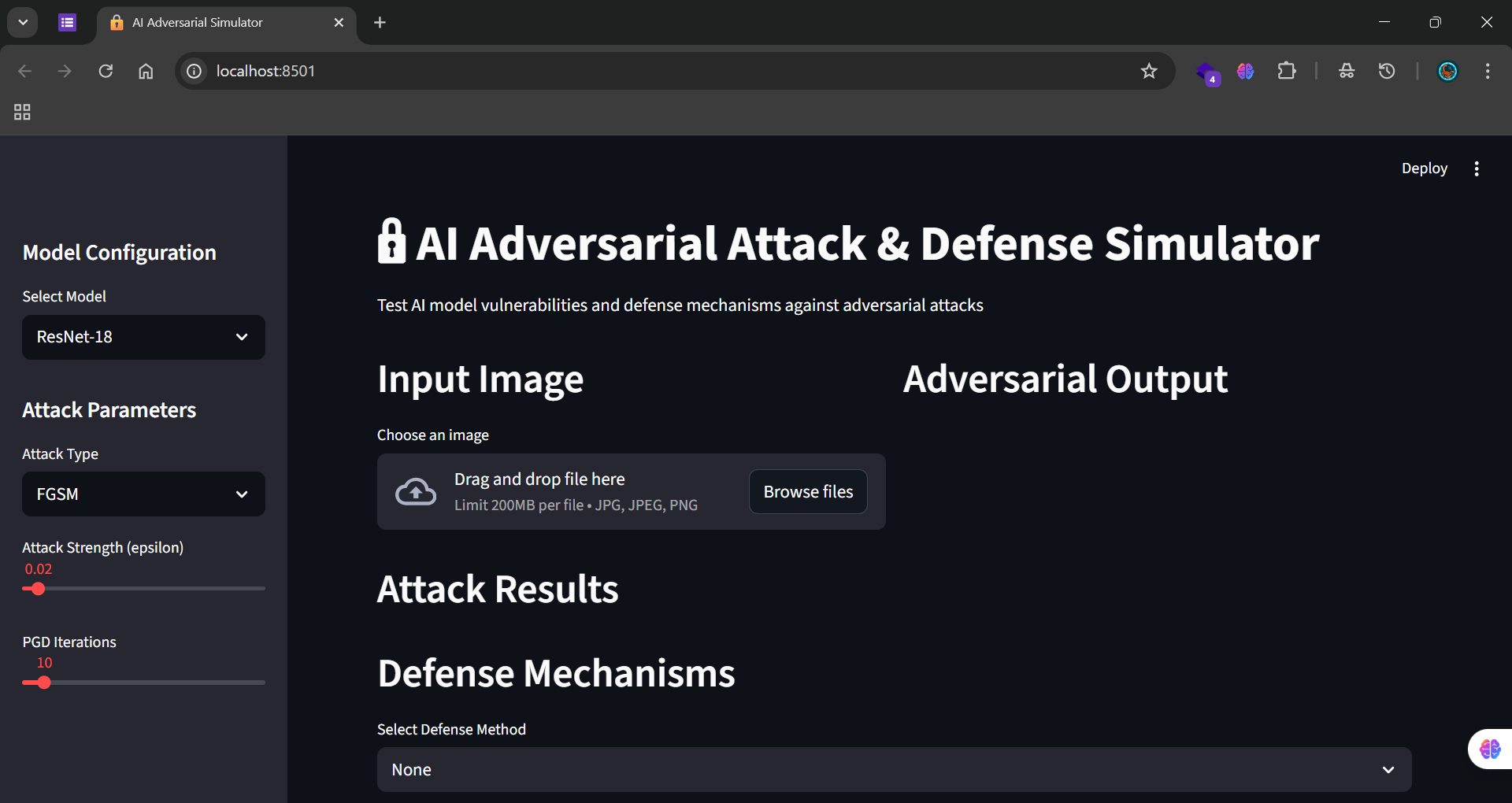
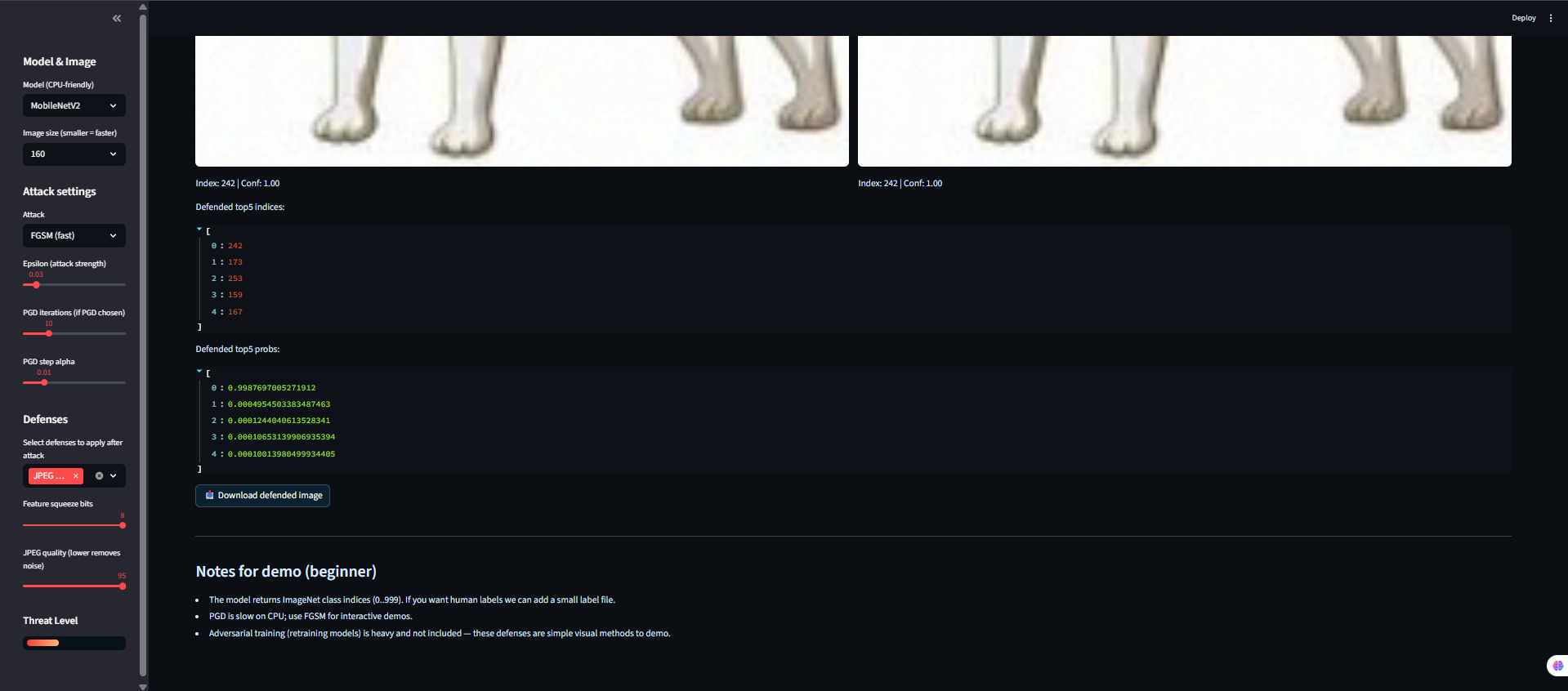
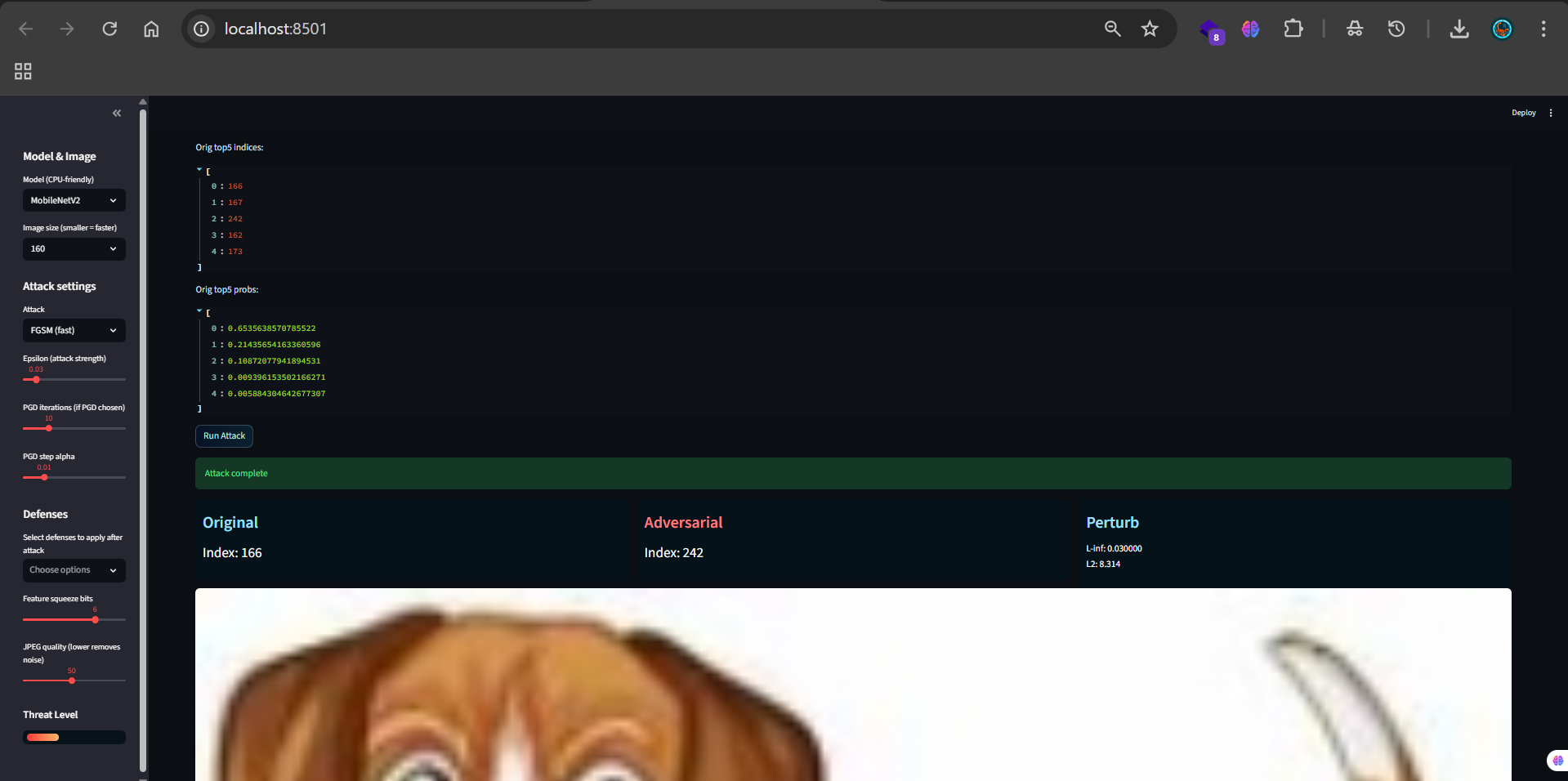
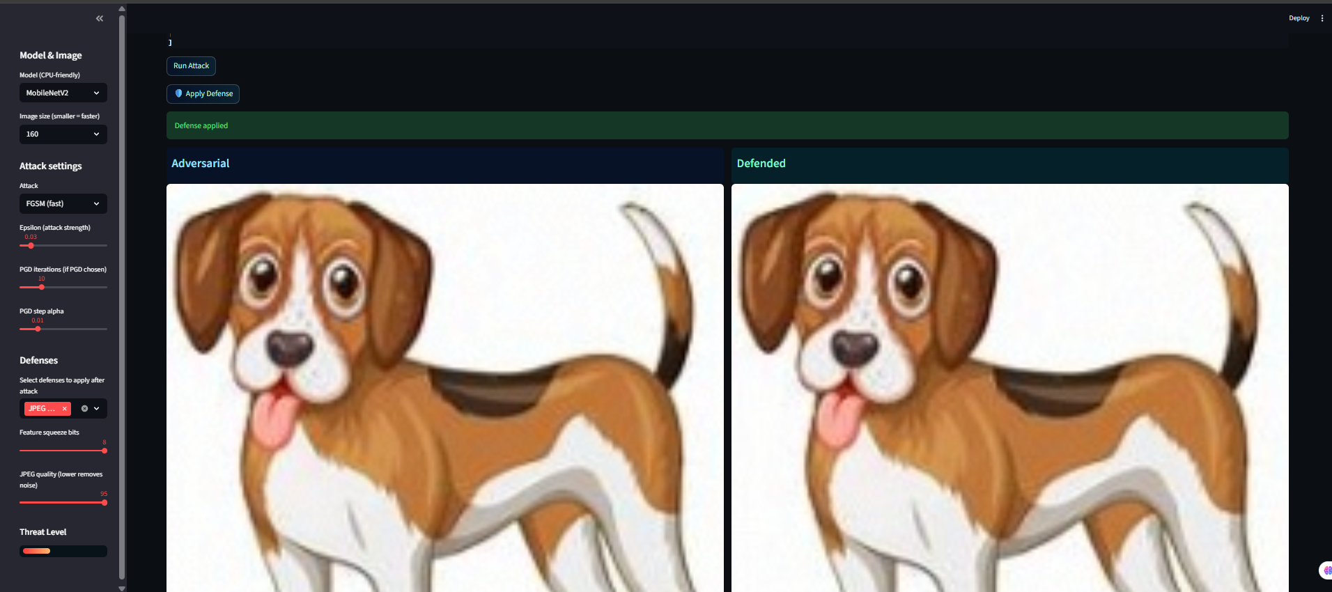
Results
| Scenario | Clean | Under attack | After defence |
|---|---|---|---|
| FGSM (ε=0.1) | ~95% | ~30% | ~78% |
| PGD (ε=0.1) | ~95% | ~12% | ~65% |
Figures are author-reported and illustrative of the observed trend, not benchmarked measurements. The consistent takeaway: weak attacks cause large accuracy drops, and defences recover a substantial (not complete) portion of that loss — with a clean-accuracy trade-off.
Limitations
- Reported accuracy figures are illustrative, not formally benchmarked with fixed seeds and held-out reporting.
- White-box first-order setting only; adaptive and black-box attacks are out of scope in this version.
Future work
- Real-time visualization dashboard (in progress).
- LLM-based adversarial attacks.
- Multi-agent Red vs Blue simulation and SOC integration.
- Docker containerization for reproducible runs.